Presentation on the topic Microsoft Excel program. Presentation "Graphic ways to submit data to Excel". History and development trends

Summary of presentations

Excel program

Slides: 35 words: 687 Sounds: 35 Effects: 54

Informatics - serious science. Decision of the settlement task. The purpose of the lesson. Lesson plan. The pictogram will allow you to download the program and start working with it. Spreadsheet. Purpose. Program capabilities. Function. Diagram. Sorting. Excel program. Everything seems to be familiar to you, but a new line appeared. When the cursor enters the cell, it becomes active. Each cell has its own address. What information can contain a cell. Data in cells have a format. Some formats are on the toolbar. Fight basic concepts. Test. Arithmetic actions. The result in this cell. - Excel.ppt program

Acquaintance with Excel

Slides: 25 words: 675 Sounds: 0 Effects: 14

Acquaintance with Excel. Purpose. File name. Running spreadsheets. Acquaintance with Excel. Acquaintance with Excel. Acquaintance with Excel. Cell. Tollbs. Main element. Numeric format. ENTER TABLE DATA. Date type. Addresses of cells. Acquaintance with Excel. Range processing functions. Acquaintance with Excel. Manipulation operations. The principle of relative addressing. Acquaintance with Excel. Line. Tableware processor. Text data. Negative meaning. Formulas. - Acquaintance with Excel.ppt

Microsoft Office Excel

Slides: 25 words: 586 Sounds: 0 Effects: 72

Outstanding, superior other. Mastering practical ways of working with information. MS Excel. Purpose. MS Excel Program objects. Diagram. Chart elements. The procedure for creating a chart. Formatting cells. Mixed reference. Link. Cell. Correct address Cells. Microsoft Office. Excel. Processing numeric data. Spreadsheet. Practical work. Microsoft Office Excel. Microsoft Office Excel. Microsoft Office Excel. Microsoft Office Excel. Microsoft Office Excel. Perfect mode. What is this. Homework. - Microsoft Office Excel.pptx

Data Table in Excel

Slides: 20 Words: 1013 Sounds: 0 Effects: 18

Table "Excel". Practical use. To acquaint with the concept of "statistics". Setting the problem and hypothesis. Initial information. Medical statistics data. Statistical data. Mathematical model. Regression model. Averaged character. Continue deals. Least square method. Parameters of functions. The sum of the squares of deviations. Write down the functions. Build a table. Linear graph. Schedule of a quadratic function. Chart regression model. Graphics. - Data Table in Excel.ppt

Microsoft Excel spreadsheets

Slides: 26 Words: 1736 Sounds: 0 Effects: 88

Analysis of spreadsheets. Consolidation. Consolidation of data. Data consolidation methods. Change the final table. Adding a data area. Change data area. Creating a relationship of the final table. Summary tables. Parts summary Table. Description of the parts of the pivot table. Summary table. Data source. Structure of the pivot table. The location of the consolidated table. Creating a table. Page fields. Masters of summary tables. External data sources. Switch. Deleting a pivot table. Updating source data. Grouping data. Charts based on pivot tables. - Microsoft Excel.ppt spreadsheets

Processing data by means of spreadsheets

Slides: 22 Words: 1878 Sounds: 0 Effects: 30

Processing data by means of spreadsheets. The structure of the table processor interface. Types of data entered. Error editing Excel. Using autofill to create rows. Non-standard row. Conditional formatting. Processing numbers in formulas and functions. Built-in functions. Examples of functions. Errors in functions. Installing links between sheets. Build diagrams and graphs. Select the type of diagram. Select data. Registration chart. Placement chart. Formatting diagram. Models and modeling. Classification of models and modeling. - Processing data by means of spreadsheets.ppt

Work in Excel

Slides: 66 words: 3302 Sounds: 0 Effects: 236

Learning to work with Microsoft. Direct view. Overview. Commands on the ribbon. What changed. What has changed and why. What is located on the ribbon. How to start working with ribbon. Groups combine all commands. Increasing the number of commands if necessary. Extra options. Place the commands on your own toolbar. Teams that are not very convenient. What happened to the previous key combinations. Keyboard shortcuts. Work with old key combinations. View of the view mode. View mode. Page fields. Work with different screen resolution. Differences. Exercises for practical classes. - Work in Excel.pptm

Formulas and functions Excel

Slides: 34 words: 1118 Sounds: 0 Effects: 190

Formula I. excel functions. What is a formula. Formulas. Rules for building formulas. Enter formula. The desired values. Press the Enter key. Excel operators. Comparison operators. Text operator. Select a cell with a formula. Editing. Types of addiction. Relative addressing. Absolute addressing. Mixed addressing. What is a function. Enter functions. Wizard features. Select a function. Arguments function. Close the window. Function categories. Category. Full alphabetical list. Date and time. Category for calculating property depreciation. The category is intended for mathematical and trigonometric functions. - Formulas and functions Excel.ppt

Logic functions Excel

Slides: 29 Words: 1550 Sounds: 0 Effects: 0

Mathematical and logical functions. Explanation of Exel. Many numbers. Syntax. Remainder of the division. Numeric value. Factor. Root. Rounds the number down. Argument. Figures on the right. Generates random numbers. The number of possible combinations. Value. Logarithm. Natural logarithm. Power. Meaning constant. Radians and degrees. Sinus corner. Cosine corner. Tangent angle. Logic functions Excel. Nested functions. Expression. Sophisticated logic expressions. Value in the cell. Truth and lies. The value may be reference. - logical functions Excel.ppt

Building graphs in Excel

Slides: 25 words: 717 Sounds: 0 Effects: 8

Building graphs in the Excel program. Microsoft Excel. Graphics. Building graphs. We specify a step in the cell. The value of the argument. Pay special attention. Correct the cell. The function is protablished. Called master diagrams. Click the "Next" button. Diagram name. Press the "Finish" button. Graph is ready. Absolute addressing cell. Building curves. Archimedean Spiral. Tab process. Steps. Automatic recalculation of data. Building a circle. X (T) \u003d R * COS (T). Build a circle. It should turn out something like this. Homework. -

Slide 1.

Clade 2.

Table view of data 1. Tables consist of columns and lines. 2. Data items are recorded at the intersection of rows and columns. Any crossing of the row and column creates a "place" to record a data called the table. 3. Data that cannot be determined by other table cells are called basic. 4. If the values \u200b\u200bof the tables of the table are determined by the values \u200b\u200bof other cells using computation. Such data is called derivatives.

Slide 3.

Spreadsheets Computer programsDesigned for storing and processing the data presented in a tabular form are called spreadsheets (the corresponding English term - Spreadsheet).

Slide 4.

Electronic excel tables One of the most popular electronic table management tools is Microsoft Excel. It is designed to work in operating windows systems 98, Windows 2000 and Windows XP.

Slide 5.

Structure excel document Each document is a set of tables - a working book, which consists of one or many working sheets. Each work sheet is called. It's like a separate spreadsheet. Excel 2003 files have extension .xls. The columns are denoted by Latin letters: A, B, with ... if the letters are missing, use two-letter designations AA, AB and Next. The maximum number of columns in the table is 256. Rows are numbered by integers. The maximum number of rows that can have table - 65536. Cells in Excel 9X are located at the intersection of columns and lines. The cell number is formed as a combination of column numbers and lines without a space between them. Thus, A1, CZ31 and HP65000 are permissible cell numbers. Excel enters the cell numbers automatically. One of the cells on the work sheet is always current.

Slide 6.

The contents of the cells from the point of view of the Excel program can contain three types of data: 1. Text data 2. Numeric data 3. If the cell contains a formula, then this cell calculated the cell content is considered as a formula if it begins with a sign of equality (\u003d). The data in the Excel program is always entered into the current cell. Before you start the input, the corresponding cell must be chosen. The current cell pointer is moved by the mouse or cursor keys. You can use such keys such as Nome, Page Up and Page Down. Pressing the keys with letters, numbers or punctuation signs automatically starts inputting data into the cell. Entered information is simultaneously displayed in the formula string. You can finish entering the Enter key by pressing the Enter key.

Slide 7.

Selection of cells in some operations can simultaneously participate several cells. In order to produce such an operation, the necessary cells must be selected. The term range is used to designate the cells group. To do this, use the reception. Stretching can be made in any direction. If you click on any cell now, the selection is canceled. Instead of stretching the mouse, you can use the SHIFT key. By clicking on the first cell of the range, you can press the SHIFT key and, without releasing it, click on the last cell. Clicking on the button in the upper left corner of the workspace allows you to select the entire leaf sheet entirely. If you select the Ctrl key when selecting the cells, you can add new ranges to the already selected one. This technique you can create even unbound bands.

Slide 8.

Cells can be removed, copy, move. 1. Pressing the Delete key does not lead to removal of the range of cells, and to clean it, that is, to deleting the contents of the selected cells. 2. In order to really remove the cells of the selected range (which is accompanied by changing the structure of the table), you need to select the range and give the command: Edit Delete. 3. By command Edit Copy or Edit Cut Clean Cells of the Selected Range dotted frame. 4. To insert the cells copied from the clipboard, you need to make the current cell in the upper left corner of the insertion area and give the Edit command to insert. 5. Copying and moving cells can also be done by dragging. To do this, you need to set the mouse pointer to the boundary of the current cell or the selected range. After it takes the appearance of the arrow, you can drag and drop. Operations with cells

Slide 9.

Creating and using simple formulas table may contain both basic and derived data. The advantage of spreadsheets is that they allow you to organize an automatic calculation of derived data. For this purpose, formulas are used in the table cells. The Excel program considers the contents of the cell as a formula if it begins with a sign of equality (\u003d). Thus, to start entering the formula into the cell, it is enough to press the "\u003d" key. However, enter formulas more conveniently, if in the formula string, click on the Edit Formula button. In this case, the formulas containing the calculated value of the specified formula opens directly under the formula string. When working with Excel, it is important not to produce any calculations "in the mind". Even if you calculate the value stored in the cell, it is absolutely difficult to use the formula.

Clade 10.

Absolute and relative addresses of cells each cell has its own address. It is uniquely determined by the number of the column and string, that is, the name of the cell. By default, the Excel program considers cell addresses as relative, that is, in this way. This allows you to copy formulas by filling. However, sometimes there are situations when when filling the cells, the formula must be saved by the absolute cell address, if, for example, it contains the value used in subsequent calculations in other lines and columns. In order to set a link to the cell as an absolute, you need to set the "$" symbol before designation. For example: a1, $ a1, and $ 1, $ A $ 1 relative cell address Absolute cell addresses

Clade 11.

Sorting and filtering data The Excel spreadsheets are often used to maintain the simplest databases. The table used as a database usually consists of several columns that are database fields. Each line represents a separate entry. If the data is presented in this form, the Excel program allows sorting and filtering. Sorting is an ordering of data ascending or descending. The easiest way to make such a sort by selecting one of the cells and clicking on the Sort by ascending or sorting descending. Sorting parameters set the Sort Data command. When filtering the database, only entries that have the desired properties are displayed. The simplest filtering means is an autofilter. It starts the Data Filter Auto Filter command. Command Data Filter Display All Allows Display All Entries. To cancel the use of the autofilter, you need to re-give the data the filter autofilter.

Slide 12.

For a more visible view of the tabular data, graphs and charts are used. Excel software allows you to create a diagram based on data from the spreadsheet, and place it in the same working book. To create diagrams and graphs, it is convenient to use the spreadsheets, designed in the form of a database. Before building a diagram, select the range of data to be displayed on it. If you enable in the range of the cells containing field headers, these headers will be displayed on the diagram as explanatory inscriptions. By selecting a data range, you need to click on the Master Charts button on the Standard Toolbar. Creating diagrams

Slide 15.

Printing a finished document Work sheets can be very large, so if you do not need to print the entire work sheet, you can define the print area. The print area is a specified range of cells, which is issued to print instead of the entire working sheet. To set the print area, you need to select the range of cells and give the file file print area set. Each work sheet in the workbook can have its own print area, but only one. If you re-give the file. The print area is set to set, then the specified print area is reset. The size of the printed page is limited to the size of the paper sheet, so even the allocation of a limited print area does not always allow to place a whole document on one printed country. In this case, there is a need to split the document on the pages. The Excel program does it automatically.

Slide 16.

Conclusion The main purpose of the spreadsheet is stored and processing numerical information. We also know the other type of tables that perform similar functions are the database tables. The main difference between spreadsheets from database tables is that they are more convenient to automatically calculate values \u200b\u200bin cells. Those cells of the cells that are entered by the user are not obtained as a result of calculations are called basic. Those data that are obtained as a result of calculations using basic data is called derivatives. There are several popular programs To work with spreadsheets. The most popular is the Microsoft Excel program running operating systems Windows.

Size: 8.6 Mgabytes
Number of slides: 20

Description Presentation Presentation Practice 5 Microsoft Excel 2010 on Slides

Acquaintance with Microsoft Excel 2010 RGKP "Kostanay state University them. A. Baitursova Department II. M Discipline: Informatics Zhambayeva A. K., teacher

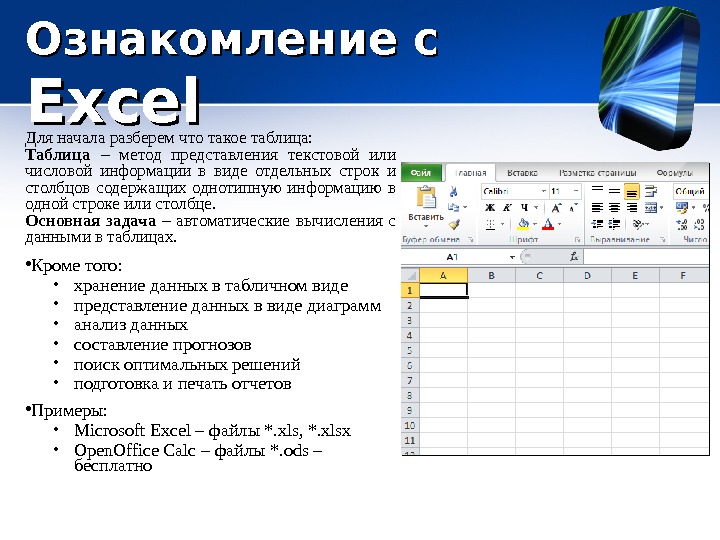
Familiarization with Excel To begin with, we will analyze what is the table: Table is a method of presenting textual or numeric information as separate rows and columns containing the same type of information in one row or column. The main task is automatic calculations with data in the tables. Also: data storage in a table view Data presentation in the form of diagrams Data analysis Drawing up Forecasts Search optimal solutions Preparing and printing reports Examples: Microsoft Excel - Files *. XLS, *. XLSX Open. Office Calc - files *. ODS - free

Acquaintance with Excel To rename the sheet Double-click on its name or select the Rename command in the context menu. To create a new sheet, click on the Distributed tab or in the context menu select the Insertion item, also in the context menu you can set the color of the label.

Entering data Entering data into the cell: To start, select the cell in which you want to insert text or the number by pressing the mouse cursor or moving the active selection with the arrow keys, then enter the text or number to save the change, press the ENTER or TAB button. When you click on ENTER, the selection moves to the string below, and when you press TAB shifted into the right. If you use the Tab key to enter data in several lines cells, and then press the Enter key at the end of this line, the cursor moves to the beginning next line. To change the already scored text, select the desired cell and press it twice with LCMs or after selecting the cell, press the F 2 key on the keyboard, and the contents can also be entered and edited in the formula string above the table.

Entering data in the cell may be displayed ##### characters if it contains information that does not fit in the cell. To see them completely, it is necessary to increase the column width. Changing column width: Option 1 1. Select the cell for which you want to change the column width. 2. On the Home tab, select the format command in the Cell Group. 3. In the Cell size menu, do one of the following. a) To fit the entire text in the cell, select the Commander Column Width. b) To increase the column width, select the column width command and enter the desired value in the column width field. Option 2 1. Move the mouse over the border of the columns in the title and perform one of the actions: a) transfer the border to the desired location, while the text hint arises with the size of the column. B) do double-click The left mouse button and the column will take the most suitable size to the content. Option 3 In the context menu of the column, select the column width and set the size.

The default data entry text does not fit into the cell takes the neighboring cell to the right of the cell. Using the transfer, you can display several lines of text inside the cell. To do this: 1. Select the cell in which the text must be transferred. 2. On the Home tab, in the Alignment group, click Transfer according to words. If the text consists of one word, it is not transferred. In order in this case, the text fit completely, you can increase the width of the column or reduce the font size. If no entire text is visible after the transfer, it may be necessary to change the height of the string. On the tab start page In the cell group, select the format, then in the Block size group, click the height of the height. Line size as well as columns can be changed the mouse cursor and calling the context menu to select the line height. To start entering data from a new line in a cell without automatic transfers, set the row rupture by pressing the Alt + Enter keys.

Filling marker Often when editing tables You must copy, cut, delete text or other information, for this you can use the same techniques as in Word, but there is still a filling marker in Excel, it is a quadrity in the angle of the active cell serves to automatically fill Cells and makes it easier to work with the program, then in the course you will understand everything, and now we will consider its main opportunities: with a selected one cell, holding for it and increasing the frame. We will copy the value of this cell to others. With the selected two cells, the program will look at their content if there is a number, then the program will continue the arithmetic progression of the difference between these numbers, and if the text, but a certain text, for example, Monday / Tuesday or January / February, the program will add to the first two Wednesday, Thursday etc. And to the second March, April, etc. Thus, it is easy to make the multiplication table by filling only four cells as shown in the figure to the right and drag the marker horizontally, then vertically.

Data formats The program automatically determines which is entered into a cell. Excel uses 13 data formats, but they define three main types: the number - if digital information is introduced not containing letters with the exception of monetary signs, the sign of the number, percentage and degree. Formula - Instructions in the form of a line record, in which the number of cell addresses (even from other sheets) can be used, as well as special words-commands that work as functions, the only thing that has a radically specifies that this formula is a sign equal at the very beginning of the line, final The format can be both a number and text. The text is what is not included in the first two definitions and is a set of letters and numbers. Still refer to the date and additional format with filling masks - telephone number, zip code, etc.

Numeric data formats - any numbers within 16 digits, the rest are rounded. Monetary - serves to calculates with cash and their presentation, when choosing a currency, its abbreviated name will automatically appear after the numbers and there is no need to dial on the keyboard, for example 120 p. or $ 10. Financial - serves to calculate the ratios of various amounts of money and has no negative values. Percentage - serves to calculate fractional values \u200b\u200band automatically exposes a percentage sign for example 0, 4 is 40%, and ½ is 50%. Fractional - the number is presented in the form of a fraction with a given divider. Exponential - serves to designate very large values, for example, 160000000000 This is 16 * 10 20 Date - date designation in various formats including days of the week. For example: 10. 06. 2003 or May 17, 1999. Time - the designation of time in different types. For example: 21: 45: 32 or 9: 45 pm. Text - just text. Additional - text having a specific writing template. For example, passport number or phone number, zip code, etc.

Data formats To set the data format in the cell you can do in the following way: On the main tab on the "Number" panel, select the desired format from the drop-down list, or click on one of the buttons of this panel according to the necessary format. Select in the context menu command the cell format and set the format manually by selecting from the list to the left, with additional options appear, such as the number of semicolons, date and time signs, etc.

Formulas formula - calculations containing numbers, mathematical signs, functions, cell names of which is taken by the number for calculations. All formulas in the table must begin with the sign equal. Cell Name Each cell has its own name, for example U 32, here u - cell column, 32 - line number, the name of the active cell is written over the table to the left line of formulas, and in MSOffice Excel 2010, the cell can be assigned another name that can be used in the formulas You just need to enter a new name in this field. There is a limit on new names - it should consist only of capital Latin letters. Functions to facilitate calculations, Excel has built-in functions, such as the root calculation, the summation of the numbers of the required cell block, etc., for adding them there is a special button allocated in the figure.

Formulas Before entering the formula, be sure to insert a sign equal! To facilitate the input to the formula table, you need to know the following techniques: To enter the address of the required cell, you can simply click on it with LKM. To insert functions, you can also use the function button located on the "Main tab" in the Editing panel or in the "Functions" tab to select the desired one. For multiple copying functions, you can use the filling marker or copying. When copying the address of the cells in the formula will be changed according to the cell in which the formula is copied. To set the unchanged cell address when copying in any way, you need to put a $ sign in front of it for example $ H $ 45 - the address is immutable both by columns and rows.

Formulas List of basic functions: sums (A 1: A 10; B 2) - the summation of the column A and cell B 2. Okrukl (number; discharge) - rounding the number to the specified number of comma numbers, similar functions of the round, and rounded. Max (A 1; in 1: at 10) - returns the maximum value from the list. If (expression; value) - Returns the "value" if the "expression" is true. SRNAVOV (A 1; in 1) - returns the average alimony value. Choice (index; zn 1; zn 2; ...) - Returns a value by "index" number degrees (rad), radians (hail) - reverse radian translation functions in degrees and back. Full list You can see the functions by clicking on the "Insert function" button and select the "Full Alphabetical List" item in the drop-down list.

Sorting data in spreadsheets provides the possibility of sorting data ascending or descending, as well as sorting over several columns at the same time. To sort one column ascending or decreasing, it is enough to select it and select one of the commands on the Data tab: Aya means "Ascending" means "descending" to sort over several columns, click the Sort button, after which you need to add the required number of columns ( levels) and set the sort order:

Sorting data as well as sorting It is necessary that only those cells that are needed to be visible to be visible is filters that can be hidden not necessary values. To add a filter, select the desired column (or a string with headers) and press the filter button in the Data tab. Using the filter, you can separate the numbers more or less specified, sort the data, hide or show certain data.

Displaying data on a sheet For ease of operation with a table Sometimes it is necessary that the title or signature of data remains visible on the screen, for this you need to highlight the string (column) below (to the right) header (signatures) and on the View tab, click the "Secure Areas" button. To view several parts of one sheet, you can use the delimiters (lines hidden near the scroll bar) - they can separate the document into four parts in each of which is displayed as part of the same sheet.

Charts and graphs are used to represent numerical information in graphical form. Charts are used to compare the same type of data, and graphics for comparing data over time or after a month or year. To create a diagram or graphics, it is necessary to create a table with data at the beginning of the table with the data that you want to display graphically, then in the Insert tab, select the most you like the diagram.

Chart All Internal Chart Elements can be reconfigured, including the type of diagram. Here is a list of variable elements: axis vertical and horizontal, mesh lines, background, bulk figures, heading, legend. Each of the elements has its own settings for configuring, this is the font, background color, dimension, position, etc.. Using the setting of these parameters, you can make a very beautiful business diagram. Settings for all elements only after their selection are called through the context menu.

Page marking in Excel Unlike Word initially, the boundaries of sheets are not displayed, so you can easily get out of the leaf. To see the borders of the sheets, you must on the "View" tab, click the "Page Markup" button. To configure the orientation of pages, scale and page size, fields on paper and page printing, we use the commands on the "Page Markup" tab. After applying the settings of the pages in the table will be separated by the dotted line of the cell divided by different sheets. To print only a certain part of the sheet, we allocate the required area and on the "Page Markup" tab, click "Print region" - "Set"

Conditional formatting (Menu on the main tab - Substitution / Supplement of numerical values graphic objects. Conditional formatting options: 1. Guest graph (on the background of numbers a diagram appears) 2. Color circuits (values \u200b\u200bare highlighted by color) 3. Icons (numbers are replaced by a set of icons)

Microsoft Excel General Information

The concept of Excel
Window program
General Workbook Information
Creating a working book
Opening working book
Saving a working book
Work sheet
Content

The concept of Excel

Excel is softwareWith which you can create tables, make calculations and analyze data. Programs of this type are called spreadsheets. In Excel, you can create tables in which automatic outcomes are calculated for entered numeric data, print beautifully decorated tables and create simple graphics.
Excel application is part of office packagerepresenting a set software products To create documents, spreadsheets and presentations, as well as to work with e-mail.
The concept of Excel

Window program
Microsoft. Excel -Program To create and process electronic tables. Microsoft Excel label most often has the form or
Microsoft Excel allows you to work with tables in two modes:
The usual is the most convenient for most operations.
Page marking - convenient for final formatting table before printing. Borders between pages in this mode are displayed in blue dotted lines. The borders of the table - a solid blue line, having flopping, which, you can change the size of the table.

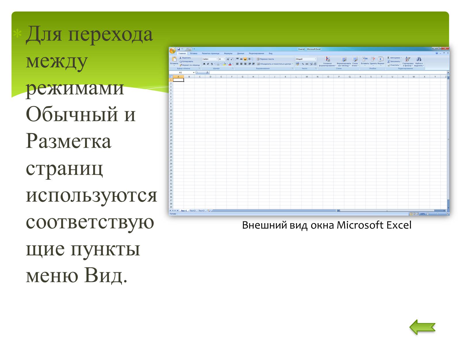
To go between the modes, the ordinary and page markup are used by the corresponding menu items view.
Appearance microsoft windows Excel

The Microsoft Excel file is called the Working Book. The working book consists of working sheets whose names (sheet1, list2, ... Usually, the default four of them are displayed on the labels at the bottom of the working book window, click on the labels, you can move from the sheet to the sheet inside the working book.
Workbook

To create a new workbook, select the Create command to select the File menu. In the template dialog box that opens, on the basis of which the workbook will be created; Then click the OK button. Ordinary working books are created based on the book template. To create a working book based on the template, you can click the button.
Creating a working book

To open an existing working book, you must select the Open or click the button on the File menu, after which the Document Opening dialog box opens. In the list field, the folder should select the disk on which the desired workbook is located. In the list below, select a folder with a book and then the book itself. According to the default, only files with Microsoft Excel books that have XLS extension are displayed. To display other types of files or all files, you must select the appropriate type in the File type list field.
Opening working book

Saving a working book

Saving a working book
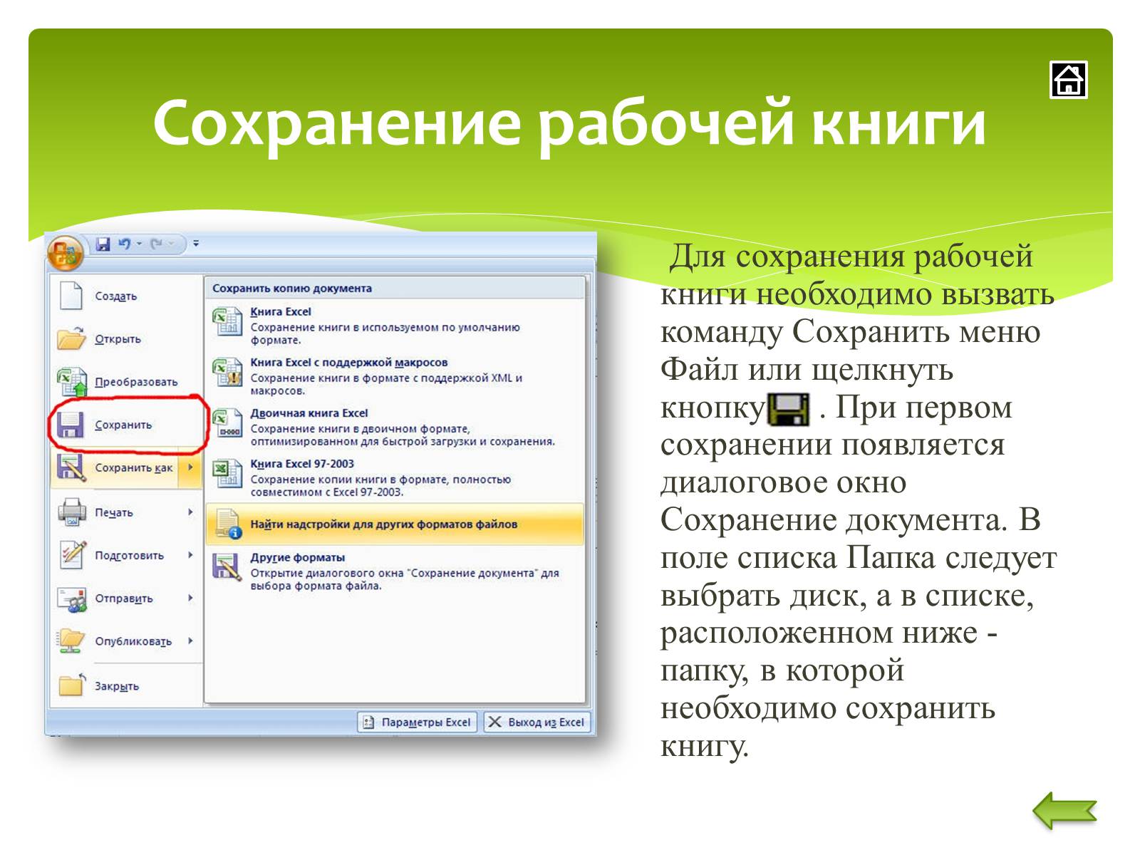
To save the working book, you must call the Save menu file command or click the button. When you first save, the Document Saving dialog box appears. In the List Field, you should select a disk, and in the list below - the folder in which you want to save the book.

Work sheet
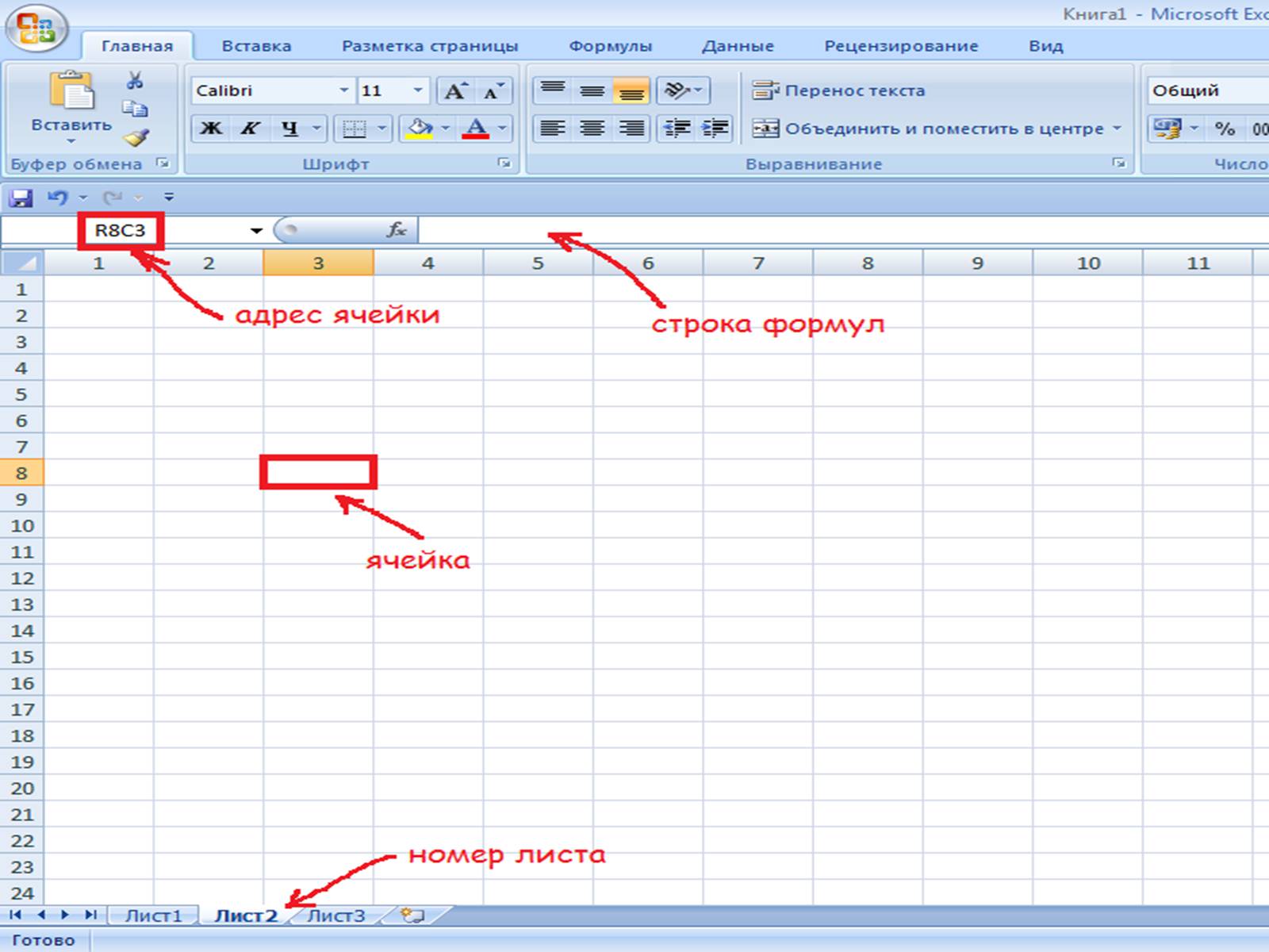
It is a table consisting of 256 columns and 65536 lines. The columns are referred to as Latin letters, and rows are numbers. Each table of the table has an address that consists of a string name and a column name. For example, if the cell is in column A and line 7, it has an A7 address. One of the tables of the table is always active. The active cell is highlighted by the frame. To make a cell active, you need to control the cursor keys to take the frame to this cell or click on the mouse.

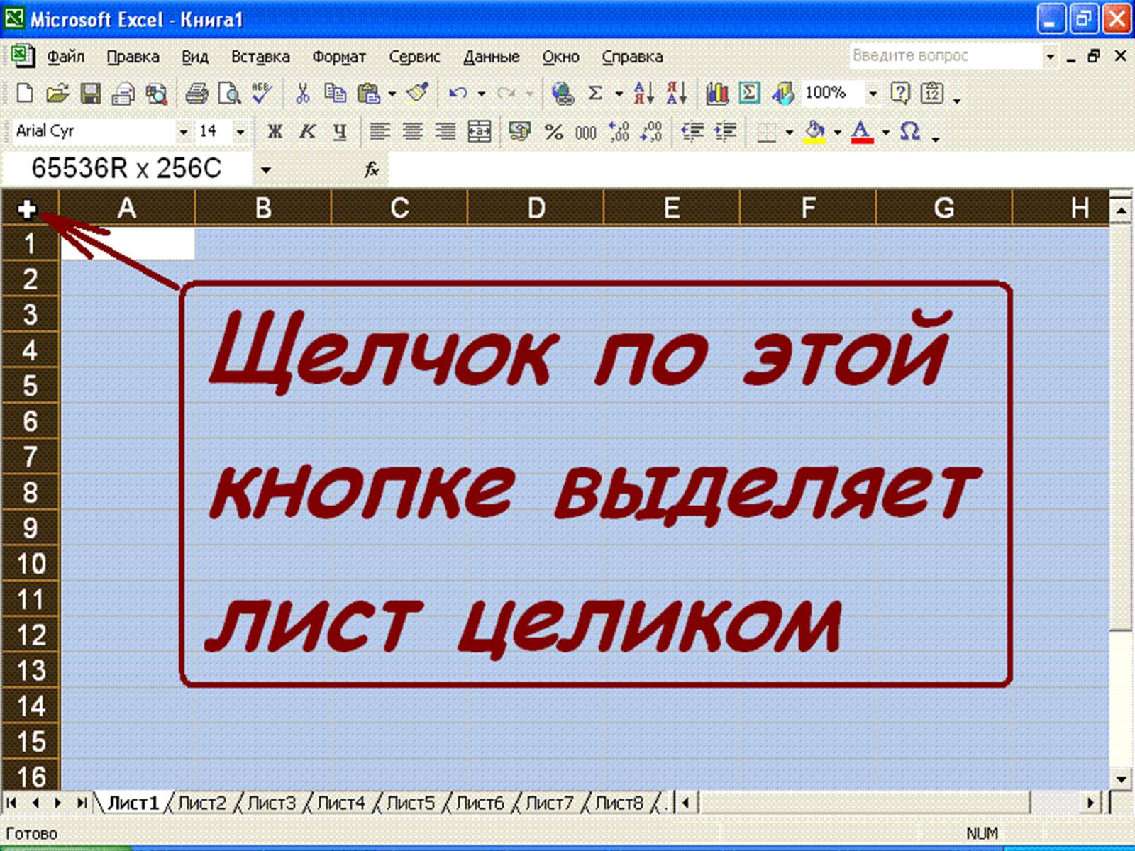
To select multiple adjacent cells, you must install the mouse pointer to one of the cells, press the left mouse button and, without releasing it, stretch the selection to the entire area. To highlight multiple non-measure groups of cells, select one group, press the Ctrl key and, without releasing it, select other cells. To select a whole column or string of the table, you need to click on its name. To select multiple columns or strings, click on the name of the first column or string and stretch the selection to the entire area.

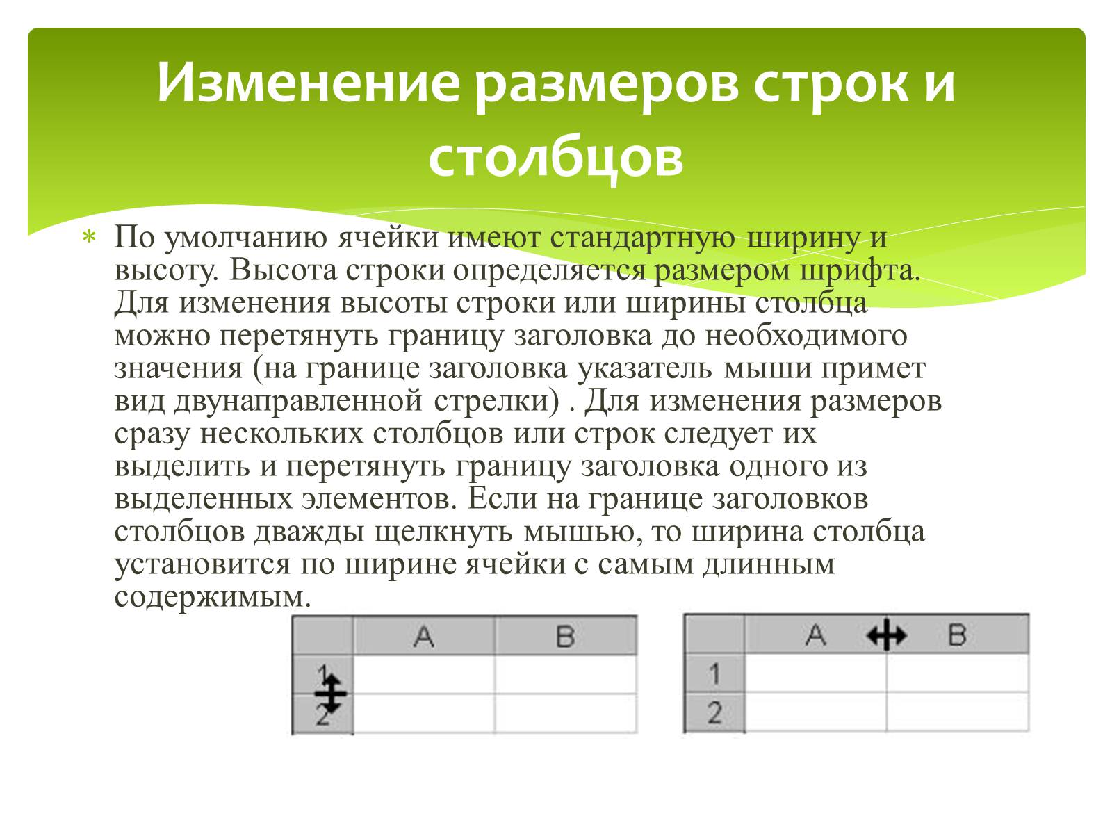
By default, cells have a standard width and height. The height of the string is determined by the font size. To change the height of the string or the column width, you can drag the header limit to the required value (on the header border, the mouse pointer will take the form of a bidirectional arrow). To change the dimensions of several columns or rows at once, it is necessary to highlight them and drag the header boundary of one of the selected items. If you double-click on the border of the header headers twice with the mouse, then the column width will be installed in the width of the cell with the longest content.
Resizing strings and columns

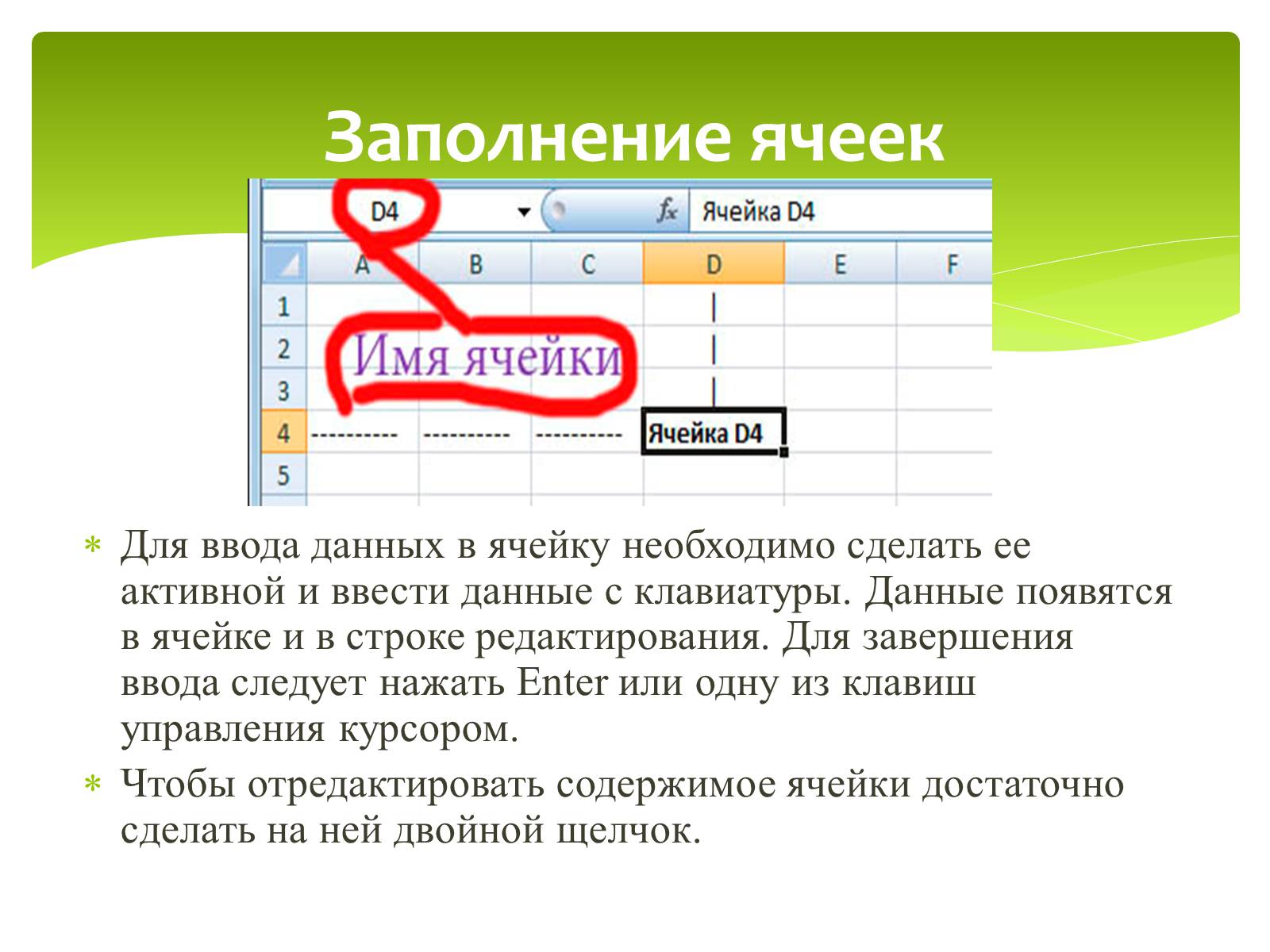
Filling cells
To enter data into the cell, it is necessary to make it active and enter data from the keyboard. The data will appear in the cell and in the editing string. To complete the input, press Enter or one of the cursor keys.
To edit the contents of the cell, it is enough to make a double click on it.

Formatting cells
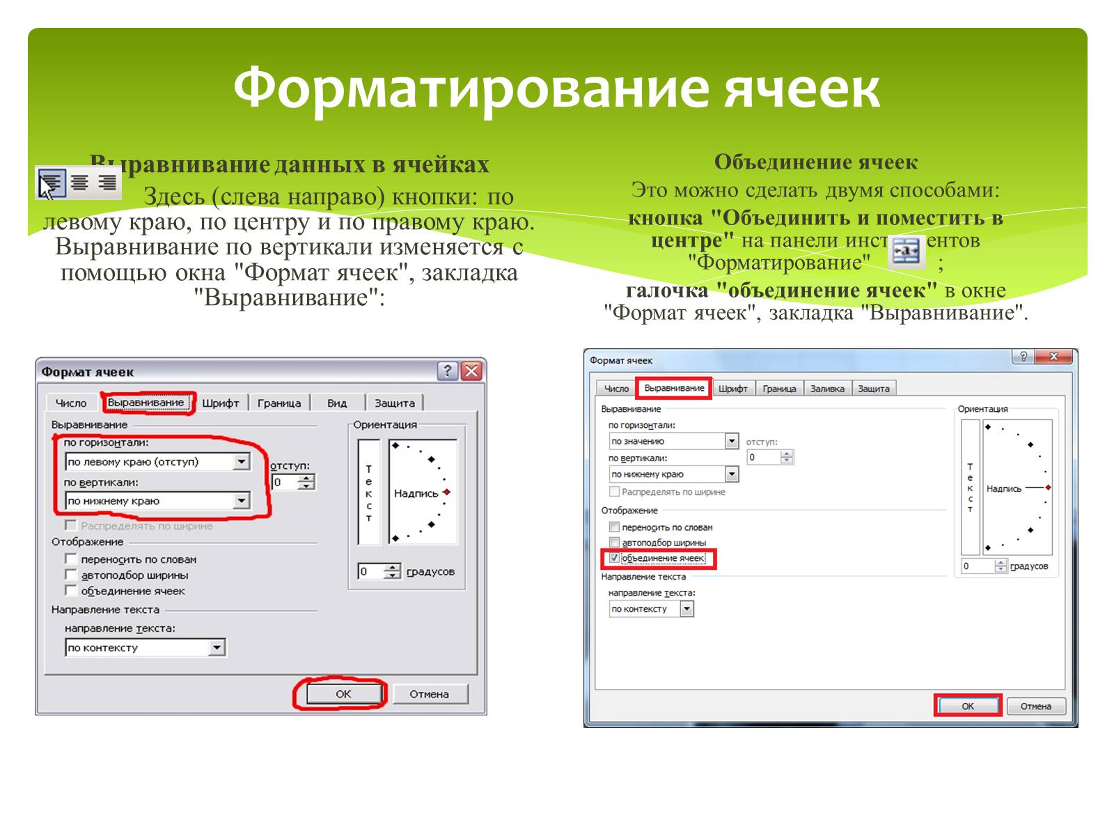
Aligning Data in Cells
Here (from left to right) buttons: on the left edge, in the center and on the right edge. Vertical Alignment Changes Using the "Cell Format" window, Alignment tab:
Combining cells
This can be done in two ways:
button "Combine and Place in the Center" on the Formatting Toolbar;
tick \u200b\u200b"Coroloring cells" in the "Cell format" window, the "Alignment" tab.

Filling of cells color
There are two ways to change the color of the fill of the selected cells:
fill color button on the formatting toolbar;
window "Format cells", "View" tab:
Adding borders of cells
Excel sheet by default presents the table. However, the table grid is not displayed until we visit them. There are three ways to add borders to selected cells:
"Border" button on the toolbar "Formatting";
window "Border", called from the "Border" button -\u003e "Draw boundaries ..."

Using dragging the filling marker * cells, you can copy its data to other cells of the same row or the same column. If the cell contains a number, date or period of time, which can be part of the row, then when copying its value is increasing.
For example, if the cell is "january", then it is possible to quickly fill out other line cells or columns by the values \u200b\u200bof February, March, etc.
Custom autocomplete lists for frequently used values \u200b\u200bcan be created, for example: a list of indicators of the activity of the library, name and position of employees, a list of divisions, etc.
Autocomplete based on adjacent cells

1. Specify the cell in which you want to enter data.
2. Dial the data and press the ENTER key.
When entering the dates, use a point or a hyphen as a separator, for example 09.05.99 or Jan-99.
Input of numbers, text, dates or time of day:

1. Enter the first cell of the range of the range and enter the initial value.
To set an increment other than 1, specify the second cell of the row and enter the corresponding value. The magnitude of increment will be set by the difference in these values.
2. Select the cell or cells containing the initial values.
3. Drag the fill marker through the filled cells.
To fill in the increasing order, drag the marker down or right.
To fill in decreasing order, drag the marker up or left.
Filling the series of numbers, dates and other elements

1. Specify the cell in which you want to enter the formula.
2. Enter \u003d (equal sign).
If you click the Change Formula or Function Insert button, the equal sign is automatically inserted.
3. Enter the formula.
Formula scheme:
4. Press the ENTER key.
Enter formula:

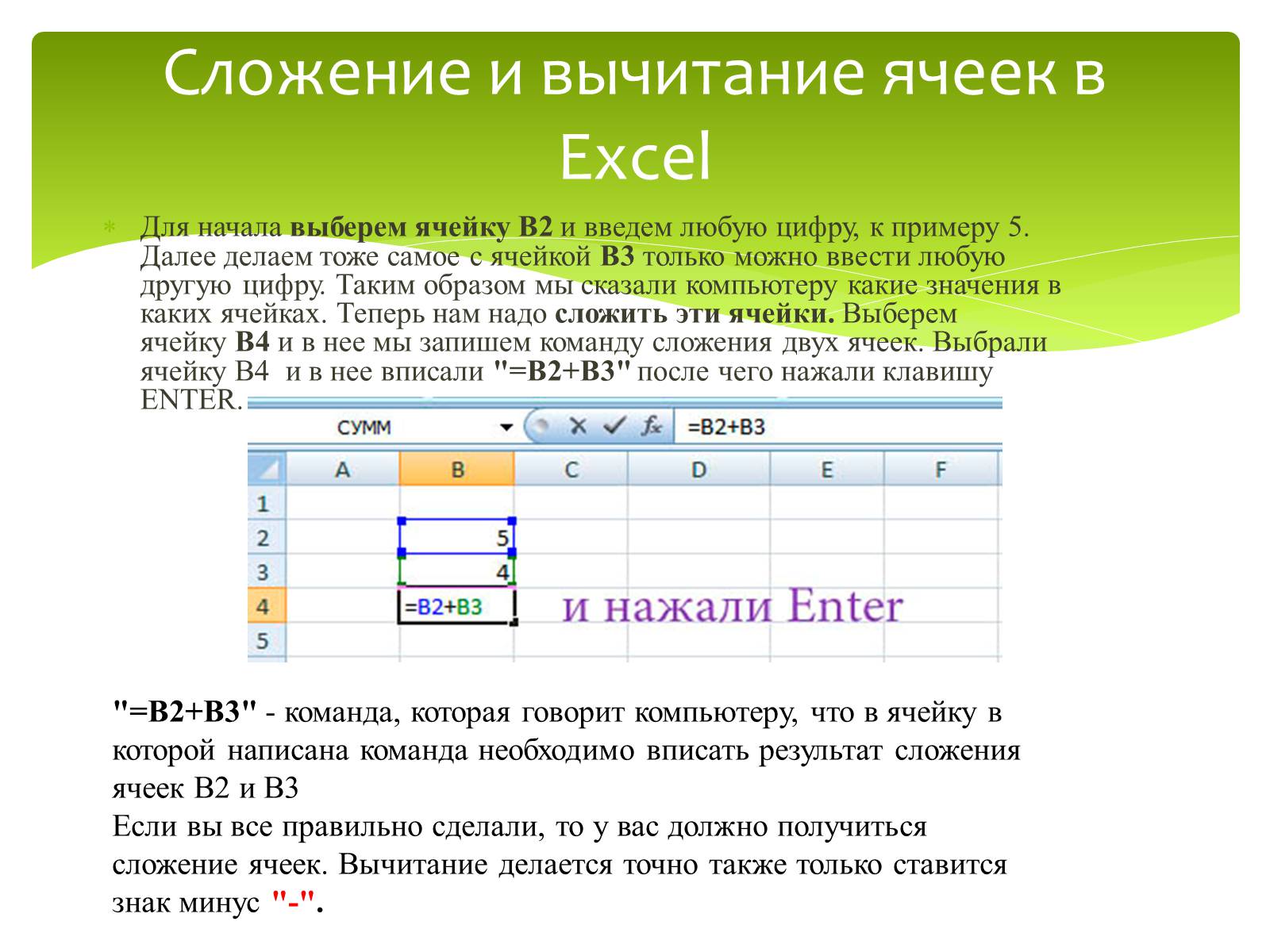
To begin with, select the B2 cell and enter any digit, for example 5. Next, we also do the same with the B3 cell, you can only enter any other digit. So we told the computer what values \u200b\u200bin which cells. Now we need to fold these cells. We choose the B4 cell and we will install the command of the addition of two cells. Chose the B4 cell and fit into it "\u003d B2 + B3" after which the Enter key was pressed.
Addition and subtraction of cells in Excel
"\u003d B2 + B3" - a command that tells the computer that in the cell in which the team is written to enter the result of the addition of cells B2 and B3
If you did everything right, then you should get the addition of cells. Subtraction is done just just put a minus sign "-".

Calculations in tables are performed using formulas. The formula may consist of mathematical operators, values, cell references and feature names. The result of the execution of the formula is some new meaning contained in the cell where the formula is located. The formula begins with the sign of the equality "\u003d". The formula can use arithmetic operators +, -, *, /. The procedure for calculations is determined by conventional mathematical laws. Examples of formulas: \u003d (D4 ^ 2 + B8) * A6, \u003d A7 * C4 + B2. etc.
Functions in Microsoft Excel are called combining several computing operations to solve a specific task. Functions in Microsoft Excel are formulas that have one or more arguments. The arguments indicate numerical values \u200b\u200bor addresses of cells. For example: \u003d sums (A1: A9) - the sum of the cells A1, A2, A3, A4, A5, A6, A7, A8, A9; for the introduction of the function in the cell: -Create the cell for formula; - Master the functions of the functions using the Insert or Buttons menu command; - in the Function Wizard dialog box, select the type of function in the category field, then the function in the function list; - lock the OK button;
Main types of action

The default header string Table includes a header string. For each column in the table in the header string, the possibility of filtering is enabled, which allows you to quickly filter or sort the data.
Microsoft Excel Table Elements

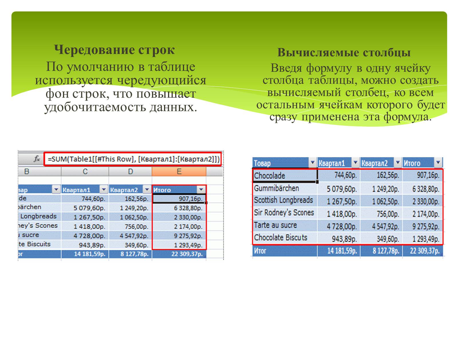
Alternating string
By default, the table is used alternating row background, which increases data readability.
Calculated columns
Entering the formula into one cell column of the table, you can create a calculated column, to all other cells of which this formula will be immediately applied.

Row of results
You can add a string of outcomes to the table that provides access to the results of summing up (for example, to the functions of the SR will, the score or sums). In each cell line, the resulting line displays the drop-down list, which allows you to quickly calculate the desired outcome values.
Size change marker
The size change marker in the lower right corner of the table allows you to drag and drop to change the size of the table.

Slide 2.

History and development trends
Basic concepts
Launch MS Excel
Acquaintance with MS Excel screen
Standard panel and formatting panel
Other Microsoft Excel Windows Elements
Work with sheets and books

Slide 3.

Appointment and scope of table processors

Practically in any field of human activity, especially when solving planning and economic tasks, accounting and bank accounting, etc. There is a need to submit data in the form of tables.
The spreadsheets are designed to store and process information provided in tabular form.

Slide 4.

Table processors provide:
input, storage and data adjustment;
design and printing of spreadsheets;
friendly interface, etc.
Modern tabular processors implement whole line Additional features:
the ability to work on the local network;
the ability to work with a three-dimensional organization of spreadsheets;
development of macros, setting the environment for the user's need, etc.

Slide 5.

History and development trends

The idea of \u200b\u200bcreating a table arose from a student of Harvard University (USA) Dan Briklin in 1979. By performing boring economic calculations with the help of an accounting book, he and his friend Bob Frankston, who understood in programming, developed the first program of the spreadsheet called by them by VisiCalc.
A new essential step in the development of spreadsheets is the appearance in 1982. On the market software Lotus 1-2-3. Lotus in the first year increases its sales volume to 50 million dollars. And it becomes the largest independent company by the manufacturer of software.

Slide 6.

The next step is the appearance in 1987. Microsoft Excel Sketch Processor. This program suggested a simpler graphic interface In combination with falling menu, expanding significantly functionality Package and enhancing the quality of the output.
Table processors available today are capable of working with you a wide range of economic and other applications and can satisfy almost any user.

Slide 7.

Basic concepts

The spreadsheet is an automated equivalent of a regular table, in the cells of which are either the data or the results of the calculation by formulas.
The workspace the electronic table consists of rows and columns having their names. Line names are their numbers. The names of the columns are the letters of the Latin alphabet.
The area is the area defined by the intersection of the column and the string of the spreadsheet having its own unique address.

Slide 8.

The address of the cell is determined by the name (number) of the column and the name (number) of the lines, on the intersection of which the cell is located.
Link - Note the address of the cell.
The cell unit is a group of adjacent cells, determined by the address. The cell block may consist of one cell, strings, column, as well as row sequences and columns.
The address is planned by an indication of the references of the first and last of its cells, between which the separation symbol is the colon or two points in a row.

Slide 9.

Meet the MS Excel tabular processor

MS Excel Tableware Processor is used to process data.
Processing includes:
carrying out various calculations using a powerful function of the function and formulas;
study of the influence of various factors on the data;
solving optimization tasks;
obtaining a sample of data satisfying certain criteria;
building graphs and charts;
statistical analysis of data.

Slide 10.

Launch MS Excel

When you start MS Excel, the Workbook "Book 1" appears on the screen containing 16 working sheets.
Each sheet is a table.
In these tables, you can store data with which you will work.

Slide 11.

MS Excel running methods

1) Starting Programs - Microsoft Office - MicrosOfTexcel.
2) In the main menu, click on "Create a document" Microsoft Office, and on the Microsoft Office panel, the Create Document icon.
The "Create Document" dialog box appears on the screen. To start MS Excel, double-click the "New Book" icon
3) Double-click on the left mouse button on a shortcut with the program.

Slide 12.

MS Excel screen

Standard panel
Formatting panel
Row of the main menu
Column headlines
String headers
Status bar
Stripes scroll
String header

Slide 13.

Field name
Row of formulas
Buttons scroll of labels
List label
Labelchkov breaking marker
Input buttons,
cancellation I.
masters functions

Slide 14.

Toolbars

Toolbars can be placed on each other in one line. For example, when the Microsoft Office application is first launched, the toolbar is standardized next to the formatting toolbar.
When placed in one bar, several toolbars may not be enough space to display all buttons. In this case, the most frequently used buttons are displayed.